This gallery is organised by intent, not by function name. Find the chart you need, copy the pipeline, adapt the aesthetics. Function-level parameters live in Reference; grammar depth lives in API.
Comparing groups
Boxplot and beeswarm
ToothGrowth |>
  plotit(encode(x = supp, y = len, fill = supp)) |>
  mark_boxplot()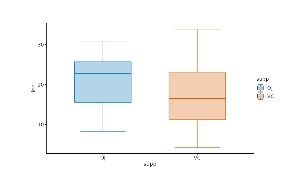
iris |>
  plotit(encode(x = Species, y = Sepal.Length)) |>
  mark_beeswarm()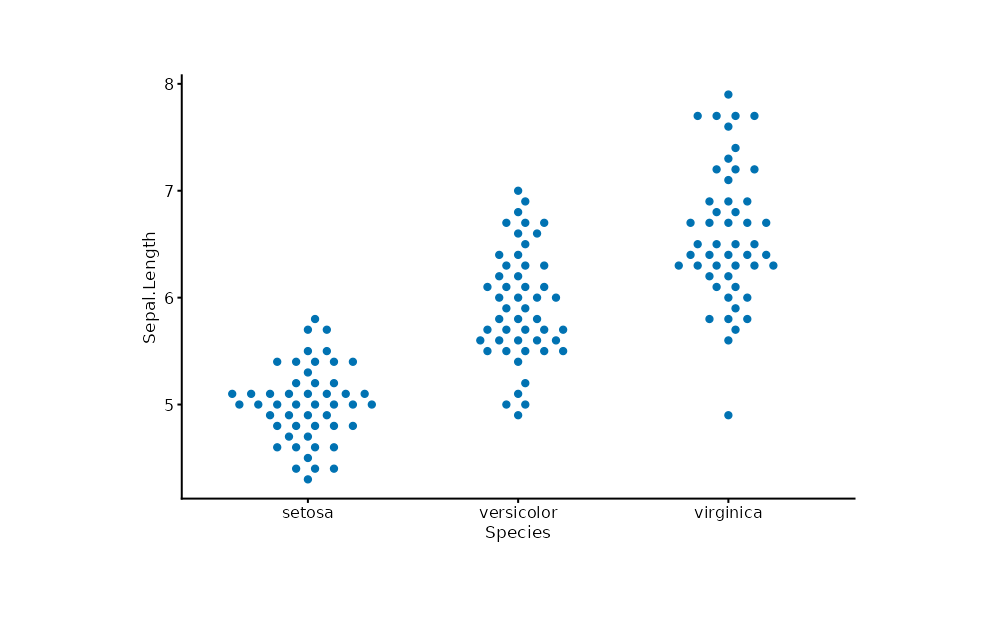
Lollipop and dumbbell
mtcars |>
  plotit(encode(x = reorder(rownames(mtcars), mpg), y = mpg)) |>
  mark_lollipop() |>
  project_cartesian(flip = TRUE)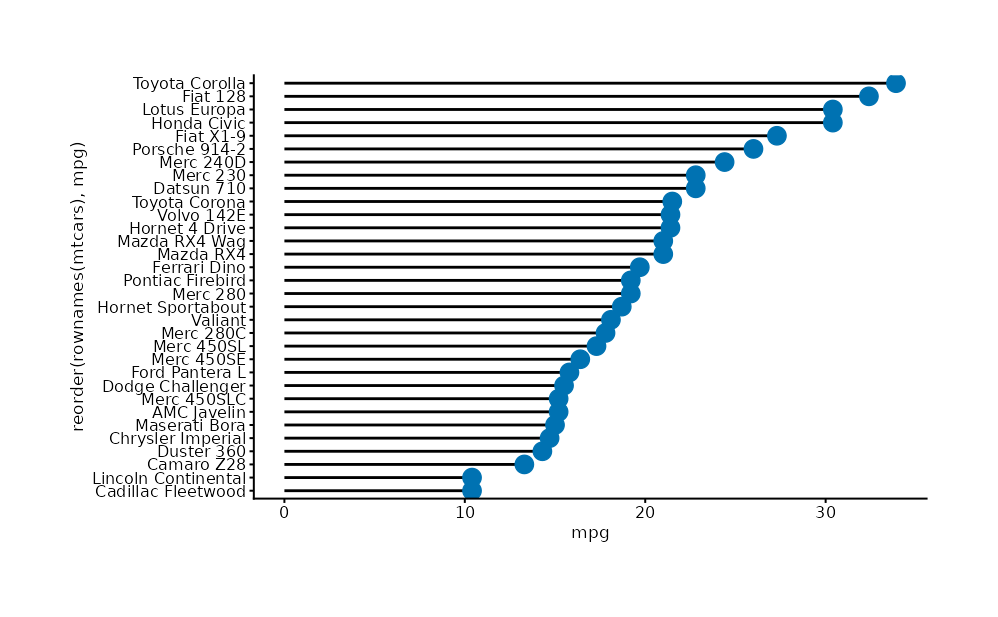
mpg_mean <- aggregate(cbind(cty, hwy) ~ class, data = ggplot2::mpg, FUN = mean)
mpg_mean |>
  plotit(encode(x = class, y = cty, yend = hwy)) |>
  mark_dumbbell()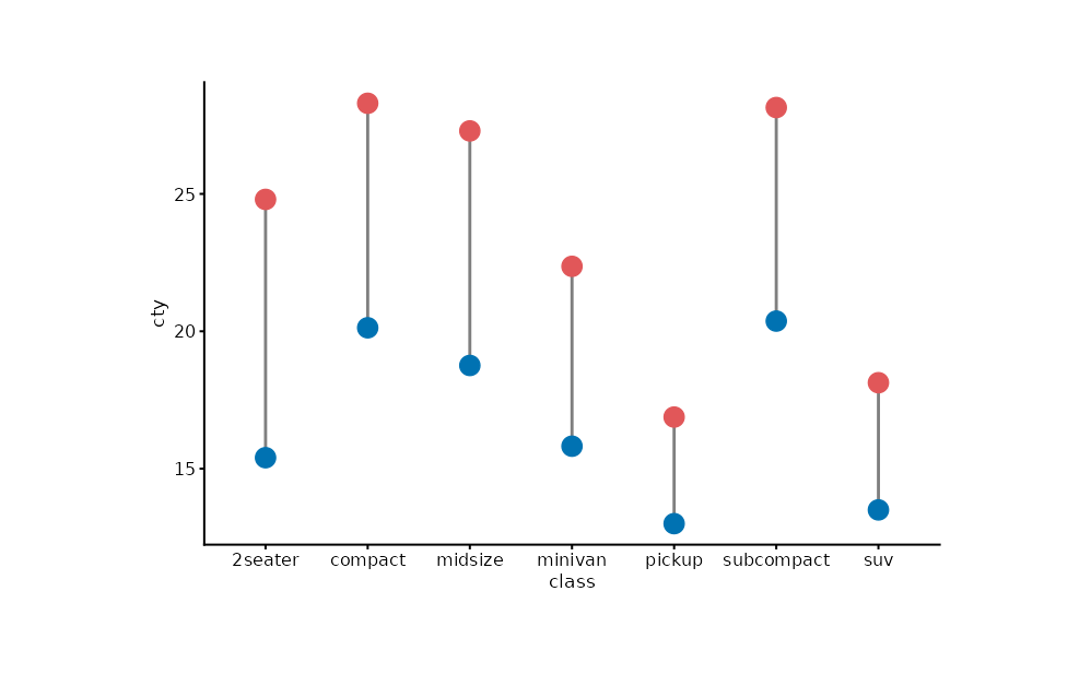
Forest plot
est <- data.frame(
  study = paste0("s", 1:5),
  est = c(0.9, 1.1, 0.8, 1.2, 1.0),
  lo = c(0.4, 0.7, 0.5, 0.9, 0.7),
  hi = c(1.6, 1.8, 1.3, 1.9, 1.4)
)
est |>
  plotit(encode(y = study, x = est, xmin = lo, xmax = hi)) |>
  mark_forest(ref = 1)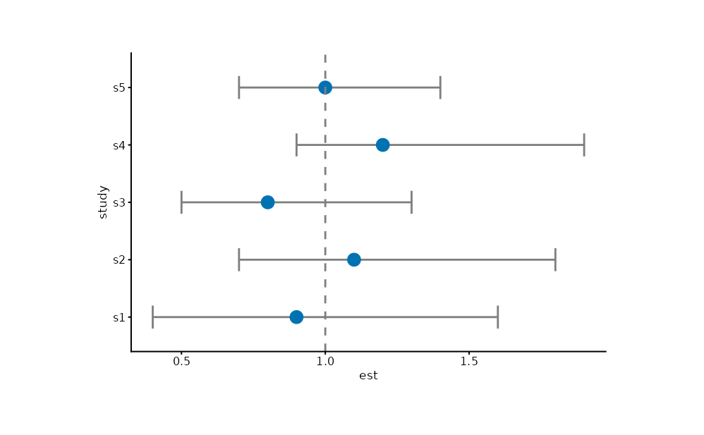
Error bars and significance
ToothGrowth |>
  plotit(encode(x = supp, y = len, colour = dose)) |>
  mark_errorbar(stat = "mean_sd", width = 0.4)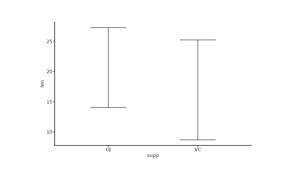
set.seed(7)
d <- data.frame(
  g = rep(c("ctrl", "A", "B"), each = 20),
  v = rnorm(60, rep(c(0, 0.8, 1.6), each = 20))
)
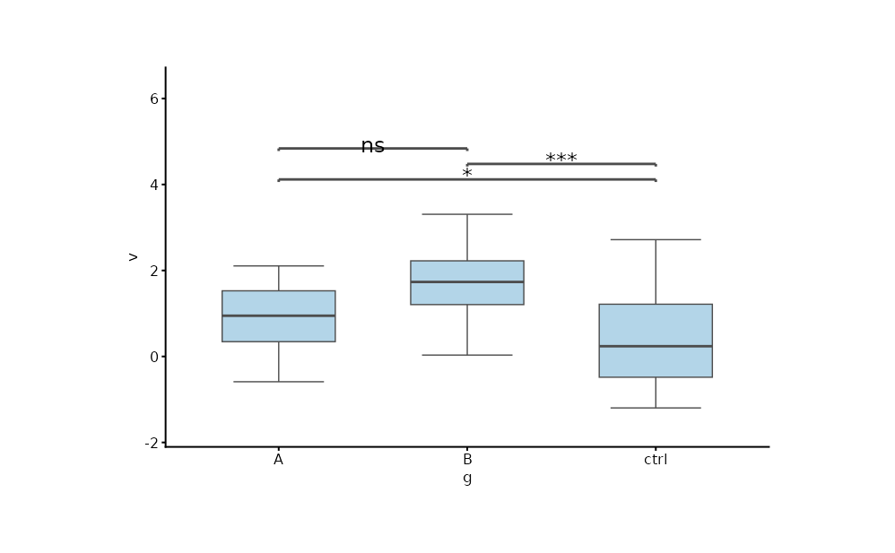
d |>
  plotit(encode(x = g, y = v)) |>
  mark_boxplot() |>
  mark_significance(comparisons = data.frame(
    group1 = c("ctrl", "ctrl", "A"),
    group2 = c("A", "B", "B"),
    label = c("*", "***", "ns")
  ))
Distributions
Histogram and density
faithful |>
  plotit(encode(x = eruptions)) |>
  mark_histogram(bins = 30)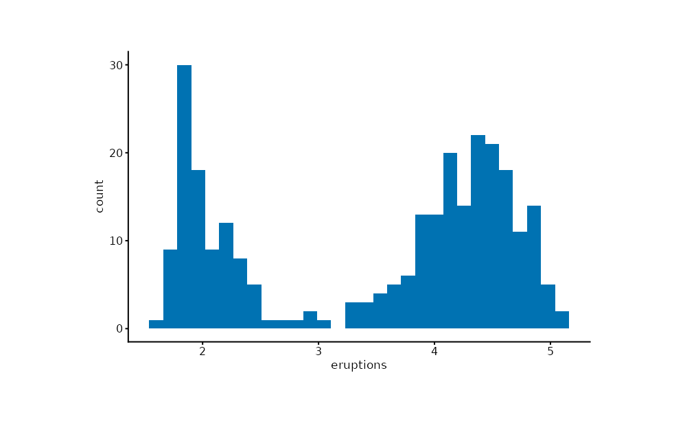
iris |>
  plotit(encode(x = Sepal.Length, colour = Species)) |>
  mark_density()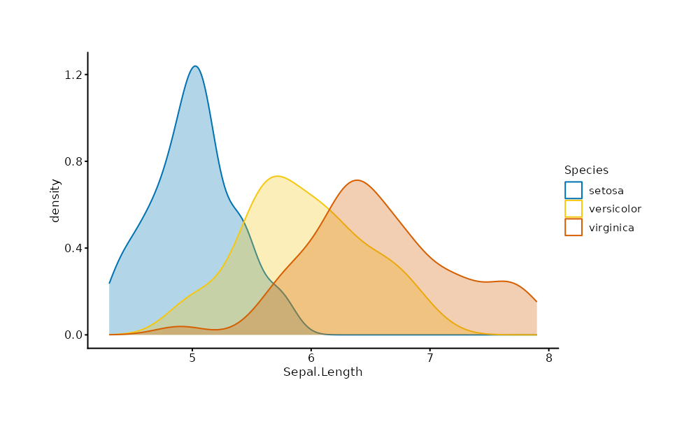
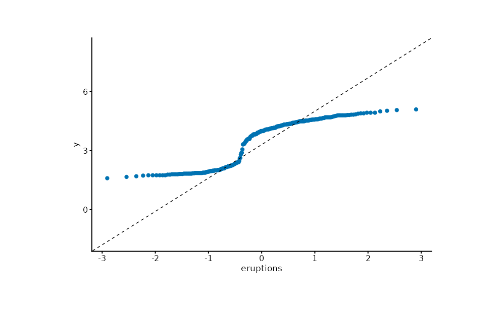
Histogram + density overlay
faithful |>
  plotit(encode(x = eruptions)) |>
  mark_histogram(mapping = encode(y = ggplot2::after_stat(density)), bins = 30, alpha = 0.5) |>
  mark_density(bw = 0.15)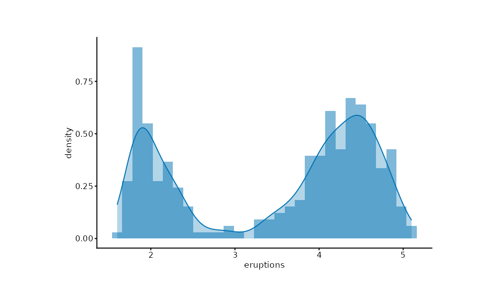
Bivariate density and binning
faithful |>
  plotit(encode(x = eruptions, y = waiting)) |>
  mark_density_2d(filled = TRUE, bins = 10)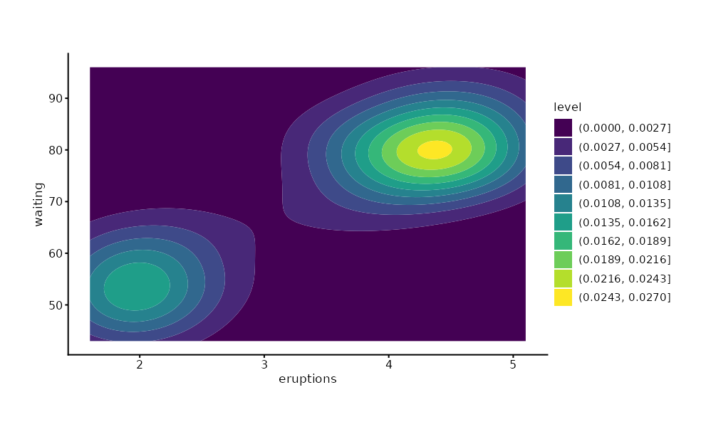
dmid <- ggplot2::diamonds[ggplot2::diamonds$carat < 2, ]
dmid |>
  plotit(encode(x = carat, y = price)) |>
  mark_hex(bins = 30)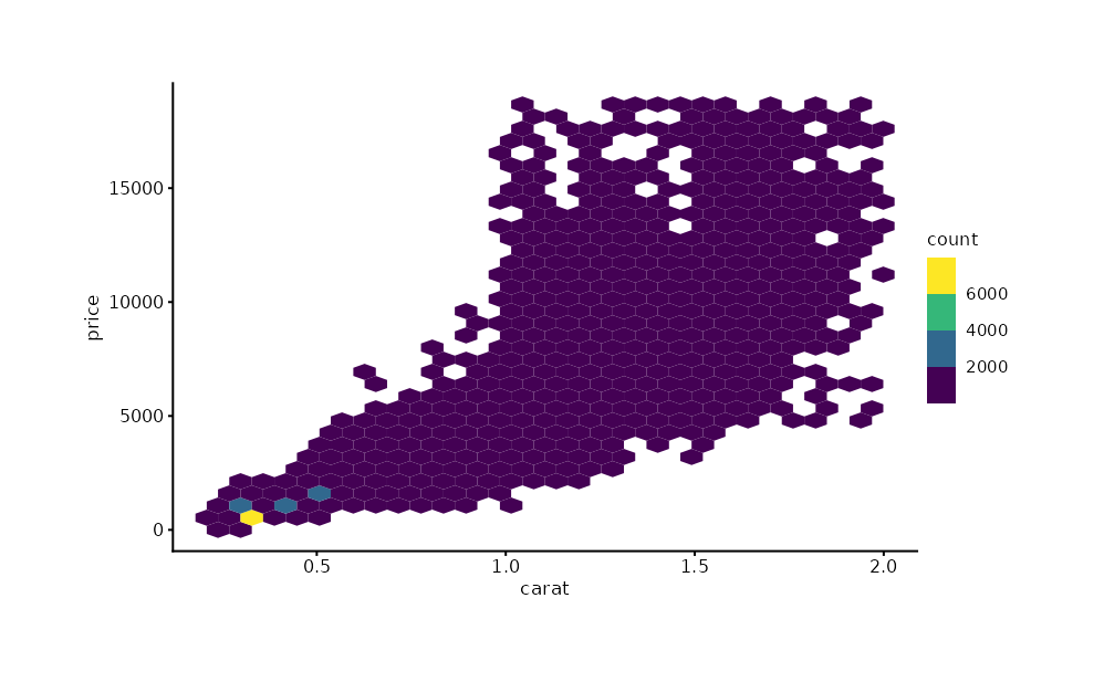
dmid |>
  plotit(encode(x = carat, y = price)) |>
  mark_bin2d(bins = 20)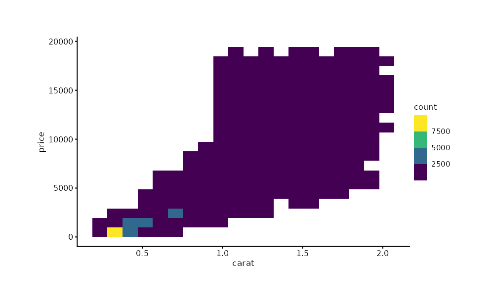
Rug ticks
faithful |>
  plotit(encode(x = eruptions)) |>
  mark_density() |>
  mark_rug(sides = "b", colour = "grey30")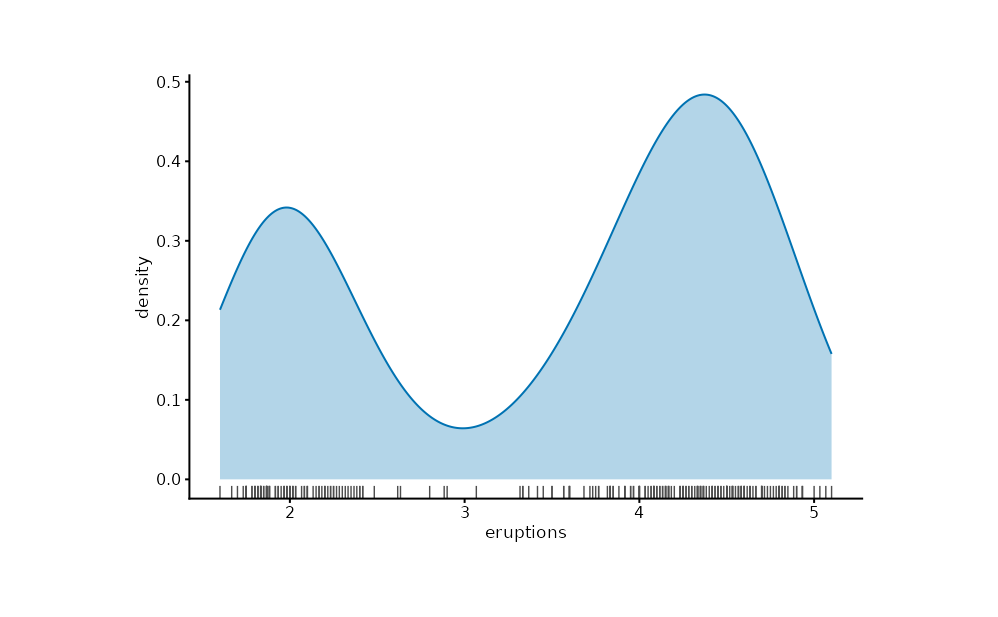
Relationships
Scatter + smooth
airquality |>
  plotit(encode(x = Temp, y = Ozone)) |>
  mark_point(alpha = 0.6) |>
  mark_smooth()
#> `geom_smooth()` using method = 'loess' and formula = 'y ~ x'
#> Warning: Removed 37 rows containing non-finite outside the scale range
#> (`stat_smooth()`).
#> Warning: Removed 37 rows containing missing values or values outside the scale range
#> (`geom_point()`).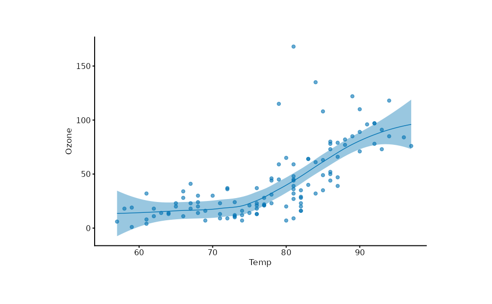
Grouped scatter
ggplot2::mpg |>
  plotit(encode(x = displ, y = hwy, colour = class)) |>
  mark_point(alpha = 0.7)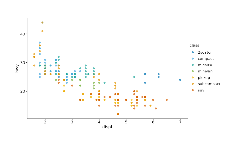
Contour of a scalar field
volcano_df <- as.data.frame(as.table(volcano))
names(volcano_df) <- c("r", "c", "z")
volcano_df |>
  plotit(encode(x = as.numeric(r), y = as.numeric(c), z = z)) |>
  mark_contour(bins = 12)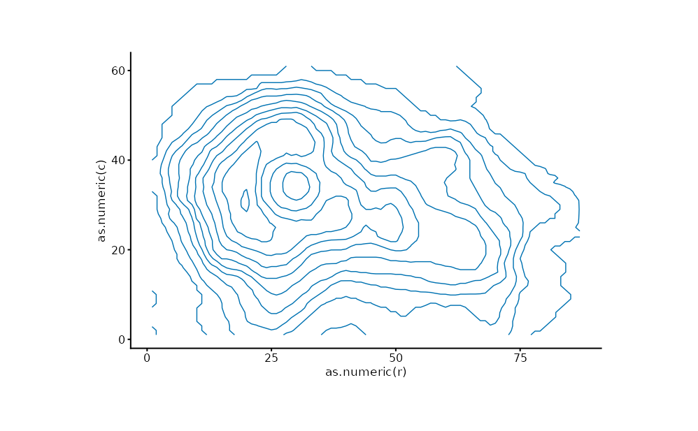
Trends
Area, ribbon, stacked area
set.seed(7)
d <- data.frame(
  x = 1:20,
  y = cumsum(rnorm(20)),
  lo = 1:20 - 1.96,
  hi = 1:20 + 1.96
)
d |>
  plotit(encode(x = x, y = y)) |>
  mark_line() |>
  mark_ribbon(mapping = encode(ymin = lo, ymax = hi))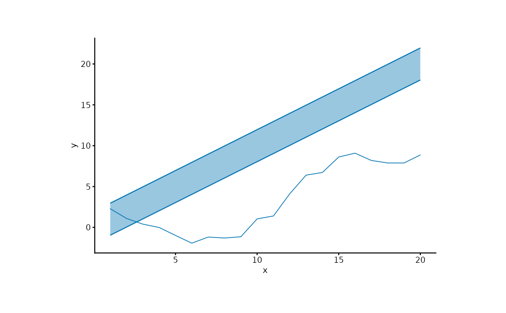
set.seed(7)
df <- expand.grid(t = 1:12, g = letters[1:4])
df$v <- rpois(nrow(df), 5)
df |>
  plotit(encode(x = t, y = v, fill = g)) |>
  mark_area(position = "stack")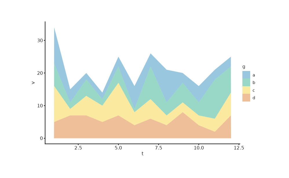
Slope chart (recipe)
sl <- data.frame(
  p = rep(c("before", "after"), each = 3),
  g = rep(letters[1:3], 2),
  v = c(3, 2, 1, 1.5, 2.5, 3)
)
sl |>
  plotit(encode(x = p, y = v, group = g, colour = g)) |>
  mark_line() |>
  mark_point()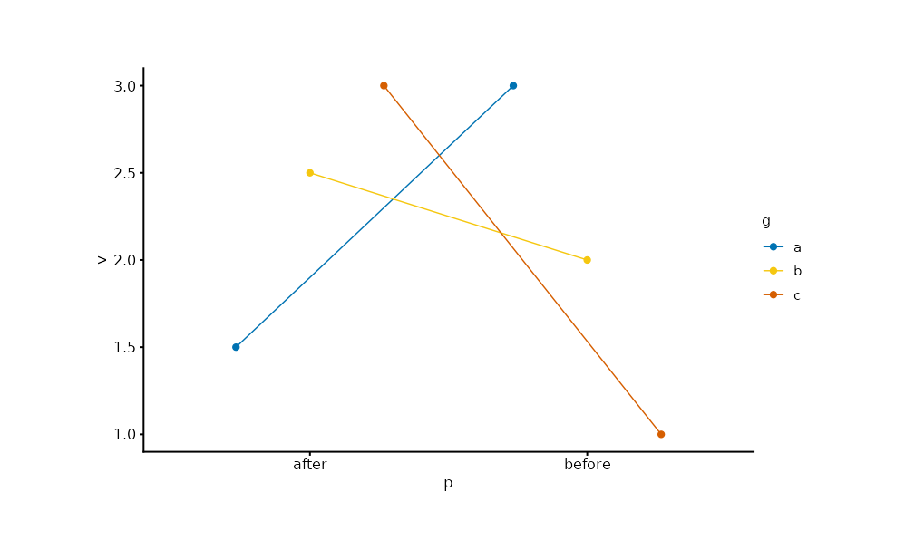
Proportions
All proportion charts are recipes: mark_bar +
project_polar.
Pie and donut
d <- data.frame(cat = c("A", "B", "C"), n = c(40, 35, 25))
d |>
  plotit(encode(x = 1, y = n, fill = cat)) |>
  mark_bar(position = "stack", width = 1) |>
  project_polar(theta = "y")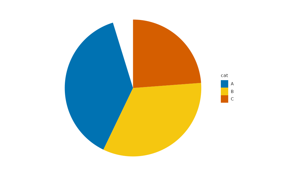
d |>
  plotit(encode(x = 1, y = n, fill = cat)) |>
  mark_bar(position = "stack", width = 1) |>
  project_polar(theta = "y", inner_radius = 0.4)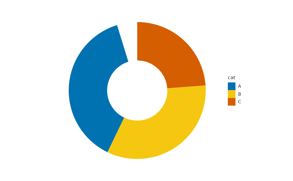
Rose / Nightingale
d |>
  plotit(encode(x = cat, y = n, fill = cat)) |>
  mark_bar(width = 1) |>
  project_polar()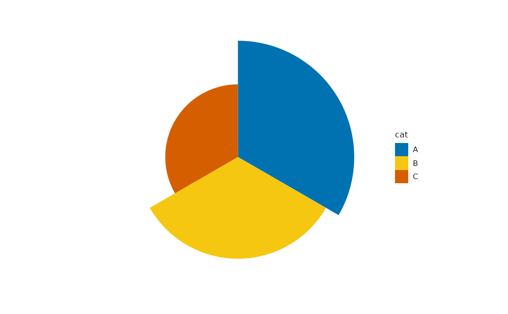
Radar (recipe)
Precompute polar coordinates, then draw polygons in Cartesian space.
set.seed(7)
lv <- 4
rd <- data.frame(
  variable = rep(letters[1:lv], 2),
  person = rep(c("p1", "p2"), each = lv),
  value = runif(lv * 2, 4, 9)
)
rd$theta <- (as.numeric(factor(rd$variable)) - 1) / lv * 2 * pi
rd$px <- rd$value * sin(rd$theta)
rd$py <- rd$value * cos(rd$theta)
rd |>
  plotit(encode(x = px, y = py, group = person, colour = person), dodge = 0) |>
  mark_polygon(alpha = 0.2) |>
  project_cartesian(fixed = 1)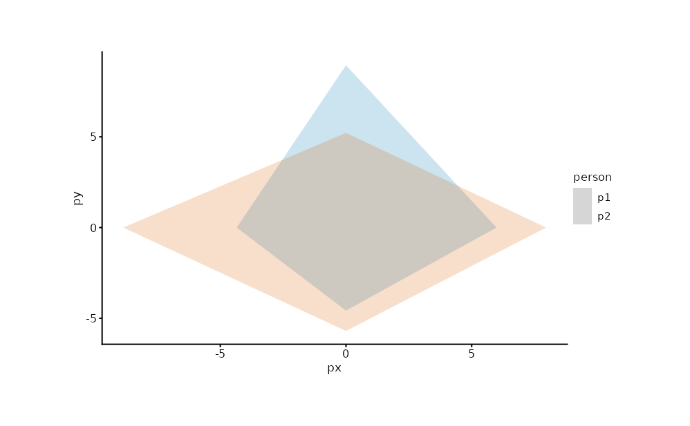
Coordinates
Flip, zoom, fixed aspect
iris |>
  plotit(encode(x = Species, y = Sepal.Length, fill = Species)) |>
  mark_boxplot() |>
  project_cartesian(flip = TRUE)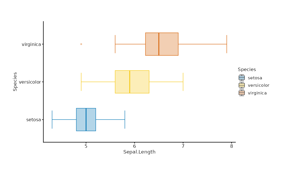
mtcars |>
  plotit(encode(x = wt, y = mpg)) |>
  mark_point() |>
  project_cartesian(xlim = c(2, 4), ylim = c(15, 25))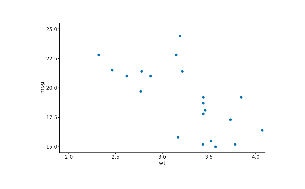
data.frame(x = rnorm(80), y = rnorm(80)) |>
  plotit(encode(x = x, y = y)) |>
  mark_point() |>
  project_cartesian(fixed = 1)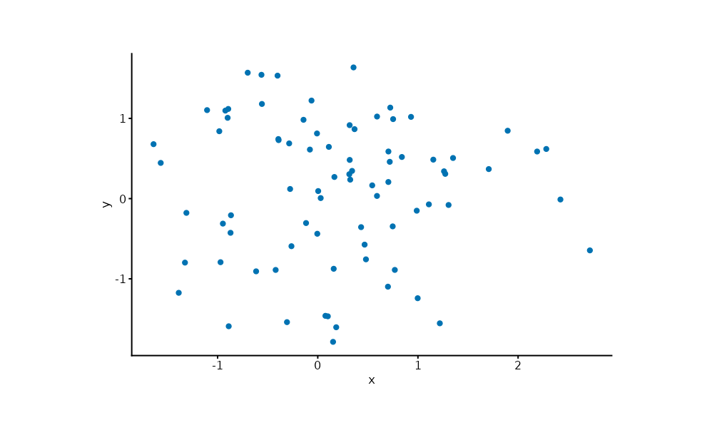
Parallel coordinates
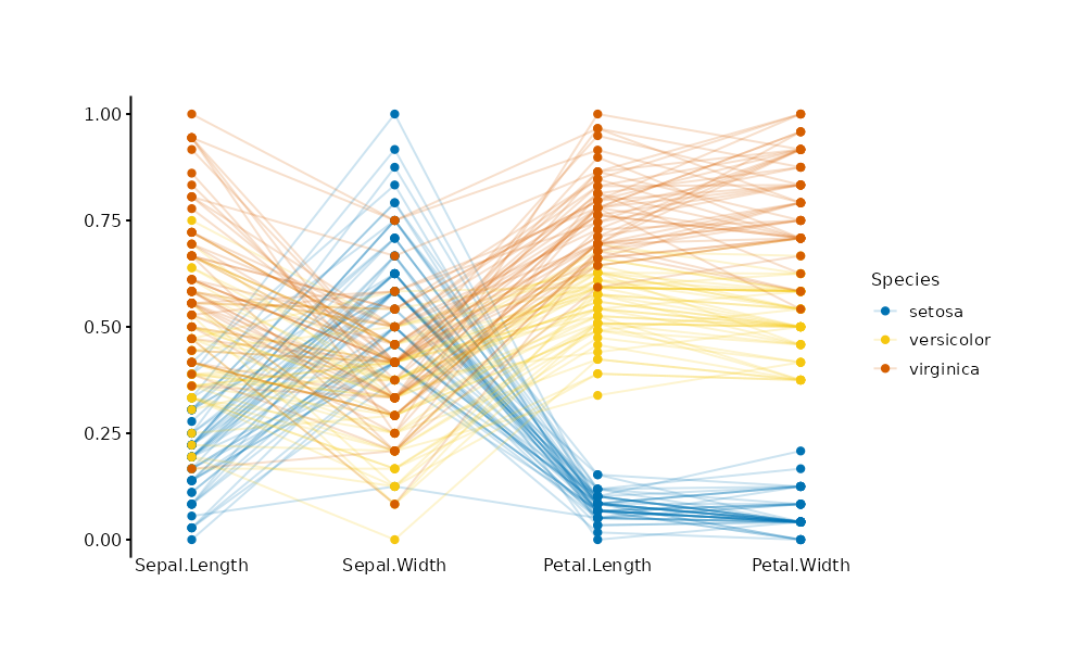
iris |>
  plotit(encode()) |>
  project_parallel(
    columns = c("Sepal.Length", "Sepal.Width", "Petal.Length", "Petal.Width"),
    group = "Species"
  )
Facets
ggplot2::mpg |>
  plotit(encode(x = displ, y = hwy)) |>
  mark_point(alpha = 0.4) |>
  split_wrap(drv, ncol = 3)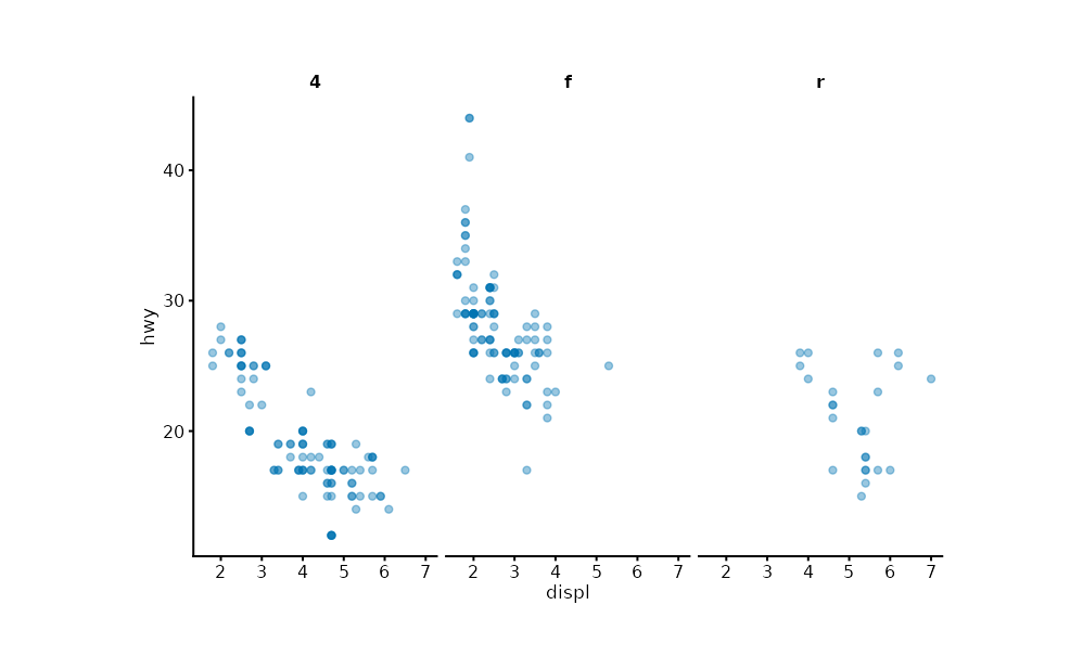
ggplot2::mpg |>
  plotit(encode(x = displ, y = hwy)) |>
  mark_point(alpha = 0.4) |>
  split_grid(drv ~ cyl)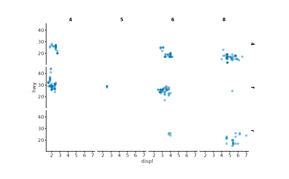
Matrix heatmaps
From long data
set.seed(7)
d <- expand.grid(r = paste0("r", 1:6), c = paste0("c", 1:6))
d$v <- rnorm(nrow(d))
d |>
  plotit(encode(x = c, y = r, fill = v)) |>
  mark_rect() |>
  scale_fill(mid = 0, range = "rdbu")
#> Scale for fill is already present.
#> Adding another scale for fill, which will replace the existing scale.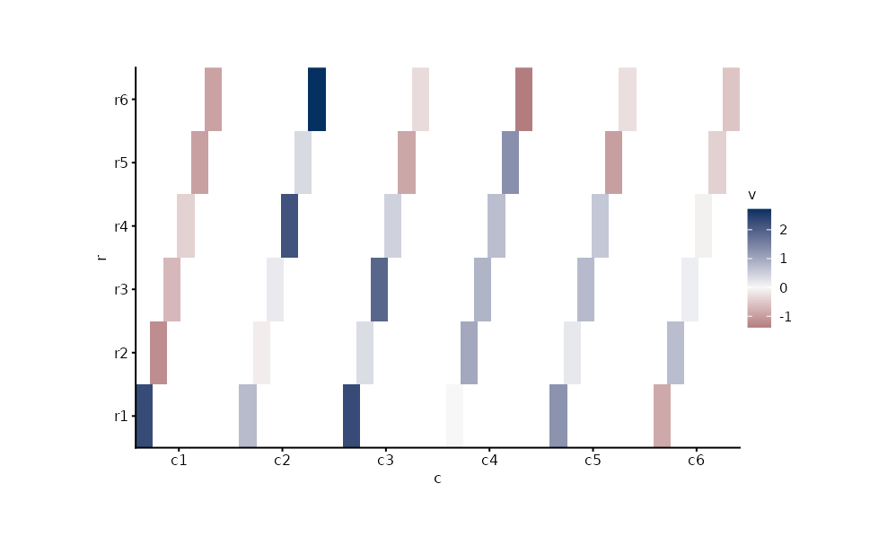
From a matrix, clustered
set.seed(7)
mat <- matrix(rnorm(48), nrow = 6, dimnames = list(paste0("g", 1:6), paste0("s", 1:8)))
h <- stats::hclust(stats::dist(mat))
plotit(mat, encode()) |>
  mark_heatmap(cluster = h, show_numbers = TRUE, number_format = "%.1f")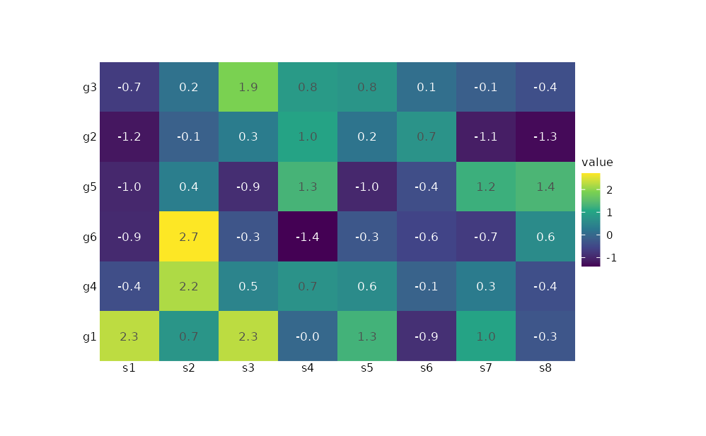
Heatmap + dendrogram (compose_annot)
hm <- plotit(mat, encode()) |> mark_heatmap(cluster = h)
tree <- as_graph(h) |>
  plotit() |>
  layout_dendrogram(direction = "up") |>
  mark_rule(data = ~edges)
hm |> compose_annot(top = tree)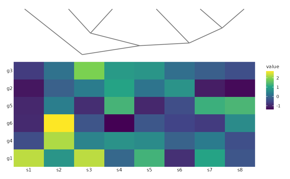
Geography
Requires sf.
if (requireNamespace("sf", quietly = TRUE)) {
  nc <- sf::st_read(system.file("shape/nc.shp", package = "sf"), quiet = TRUE)
  nc |>
    plotit(encode(fill = AREA)) |>
    mark_map() |>
    scale_fill(range = "viridis") |>
    project_map()
}
#> Scale for fill is already present.
#> Adding another scale for fill, which will replace the existing scale.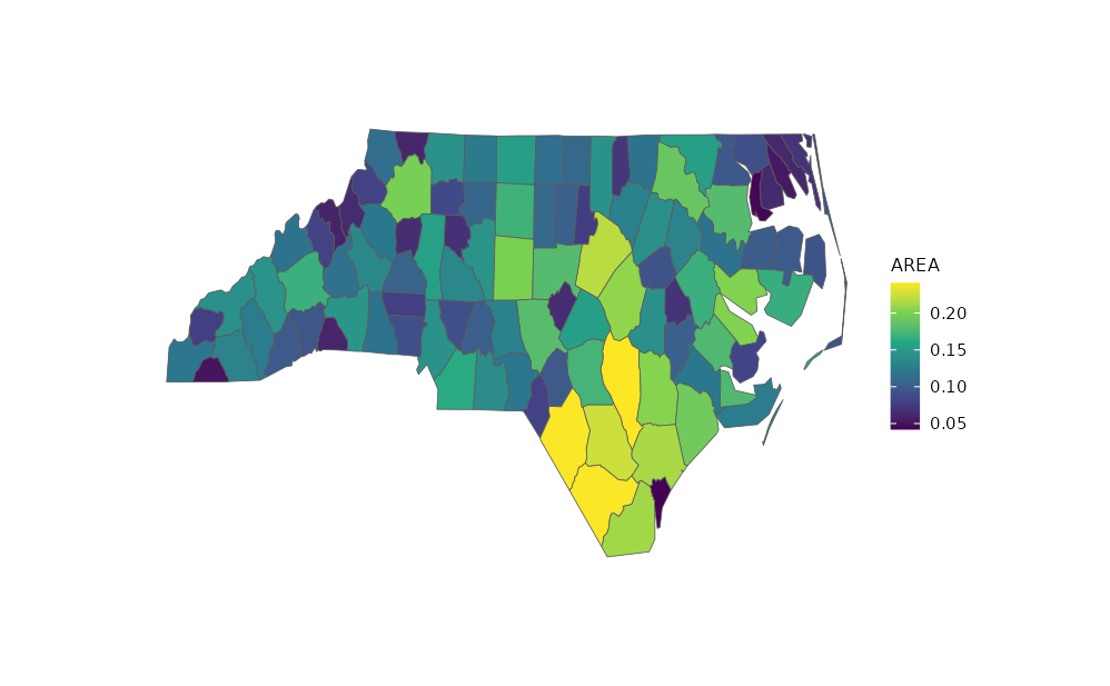
Networks and flows
Sankey
flows <- data.frame(
  source = c("A", "A", "B", "B", "C"),
  target = c("B", "C", "C", "D", "D"),
  value = c(10, 5, 8, 3, 6)
)
flows |>
  plotit(encode(source = source, target = target, value = value, fill = source)) |>
  mark_sankey()
#> Coordinate system already present.
#> ℹ Adding new coordinate system, which will replace the existing one.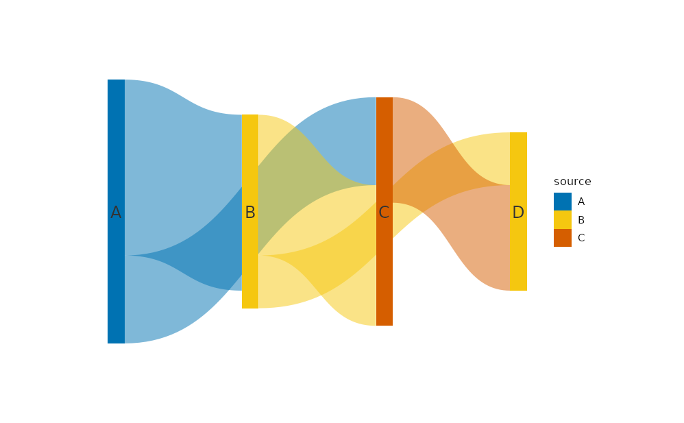
Treemap
tree_df <- data.frame(
  id = c("root", "a", "b", "a1", "a2", "b1"),
  parent = c(NA, "root", "root", "a", "a", "b"),
  value = c(NA, NA, NA, 30, 20, 50)
)
tree_df |>
  plotit(encode(fill = id)) |>
  mark_treemap()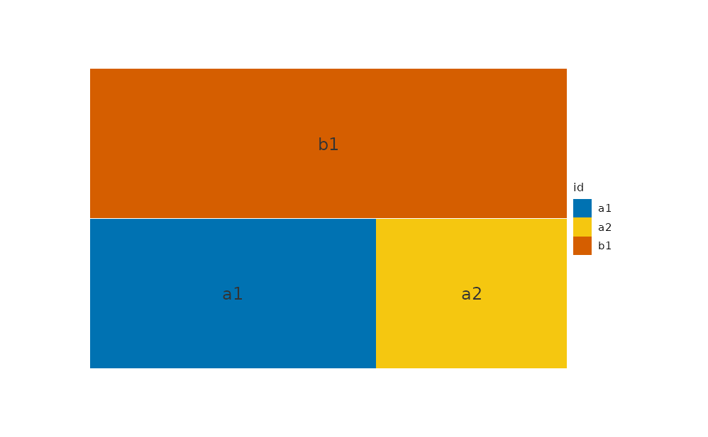
Network
nodes <- data.frame(id = c("a", "b", "c", "d"), type = c("x", "y", "x", "y"))
edges <- data.frame(source = c("a", "a", "b", "c"), target = c("b", "c", "c", "d"))
nodes |>
  plotit(encode(colour = type, label = id)) |>
  mark_network(edges = edges, seed = 4)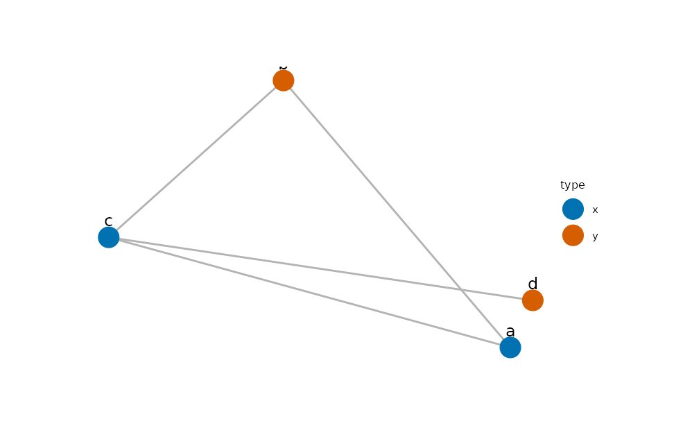
Chord
m <- matrix(c(0, 5, 2, 3, 5, 0, 4, 1, 2, 4, 0, 6, 3, 1, 6, 0), 4,
  dimnames = list(letters[1:4], letters[1:4])
)
as_graph(m) |>
  plotit() |>
  layout_chord() |>
  mark_polygon(data = ~ribbons) |>
  mark_polygon(data = ~arcs)
Tree / dendrogram
as_graph(hclust(dist(iris[, 1:4]))) |>
  plotit() |>
  layout_dendrogram(direction = "down") |>
  mark_rule(data = ~edges) |>
  mark_point(data = ~nodes)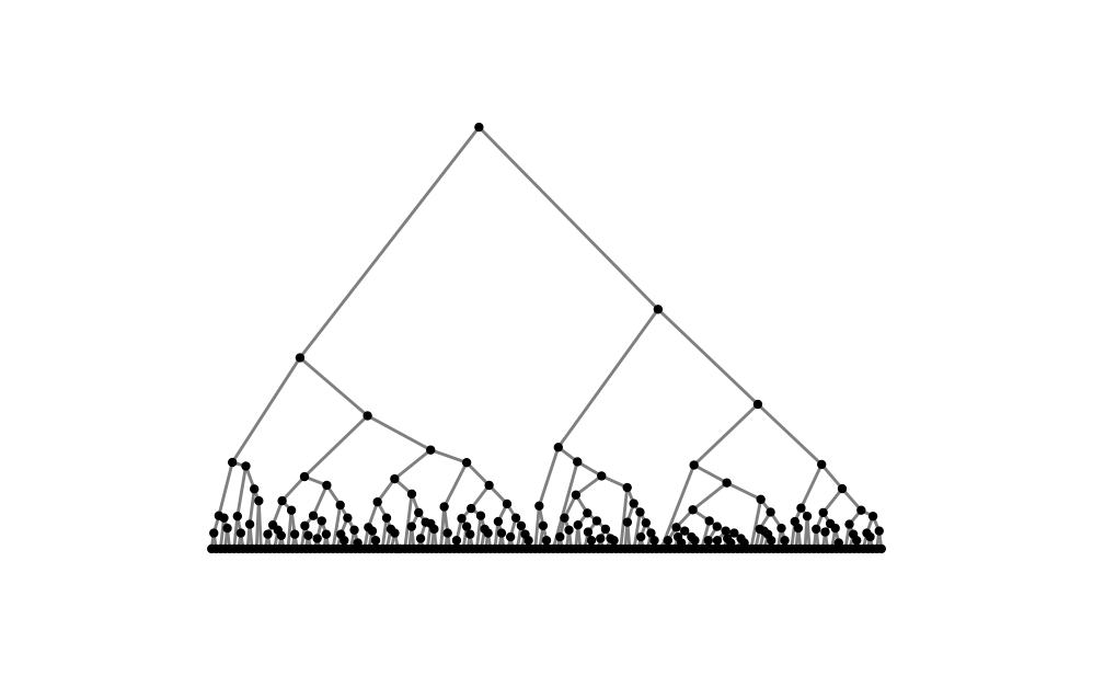
Annotations
Reference lines, labels, encircle
ggplot2::mpg |>
  plotit(encode(x = displ, y = hwy)) |>
  mark_point(alpha = 0.5) |>
  mark_rule(yintercept = 25, colour = "#E15759")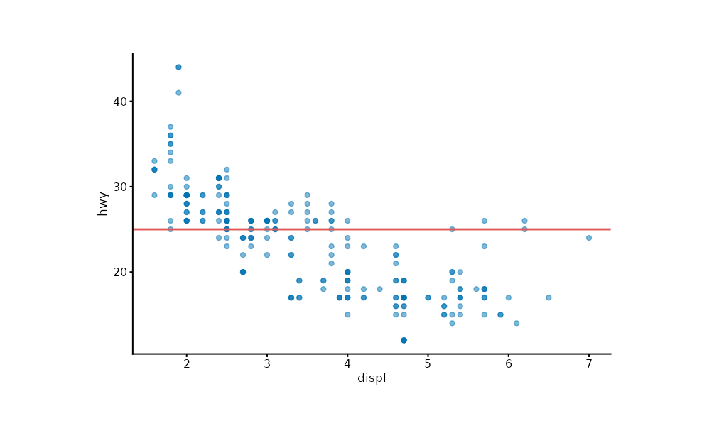
set.seed(7)
pts <- data.frame(
  x = rnorm(60), y = rnorm(60),
  g = rep(letters[1:3], each = 20)
)
pts |>
  plotit(encode(x = x, y = y, colour = g)) |>
  mark_point(alpha = 0.6) |>
  mark_encircle(shape = "hull", expand = 0.02)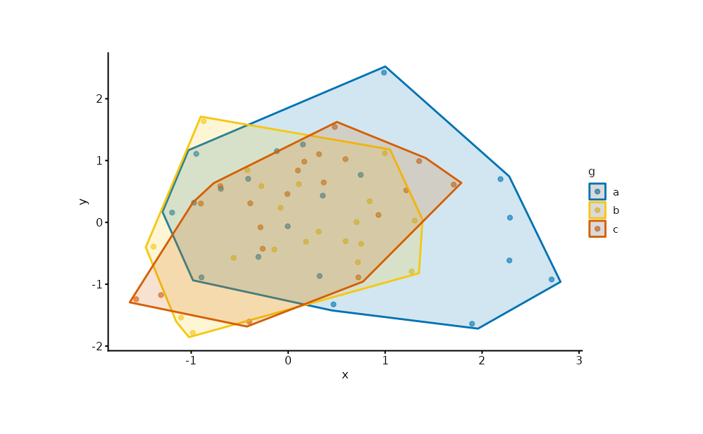
lab <- data.frame(x = c(1, 2, 3), y = c(3, 1, 2), label = c("peak", "dip", "mid"))
lab |>
  plotit(encode(x = x, y = y, label = label)) |>
  mark_point() |>
  mark_text(repel = TRUE)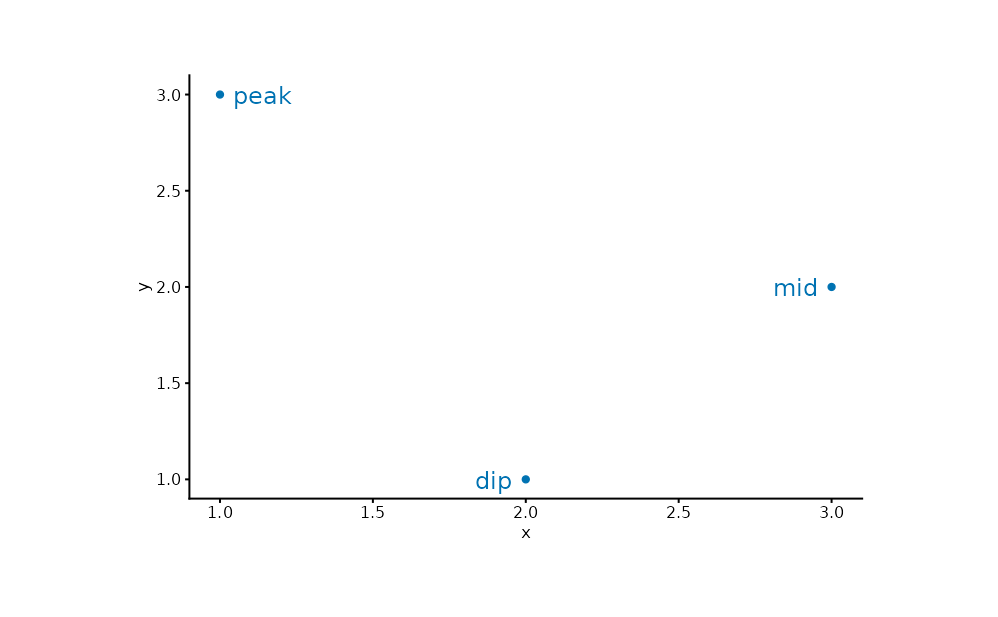
Colour scales
mtcars |>
  plotit(encode(x = wt, y = mpg, colour = hp, size = hp)) |>
  mark_point() |>
  scale_color(range = "viridis") |>
  scale_size(range = c(1, 9))
#> Scale for colour is already present.
#> Adding another scale for colour, which will replace the existing scale.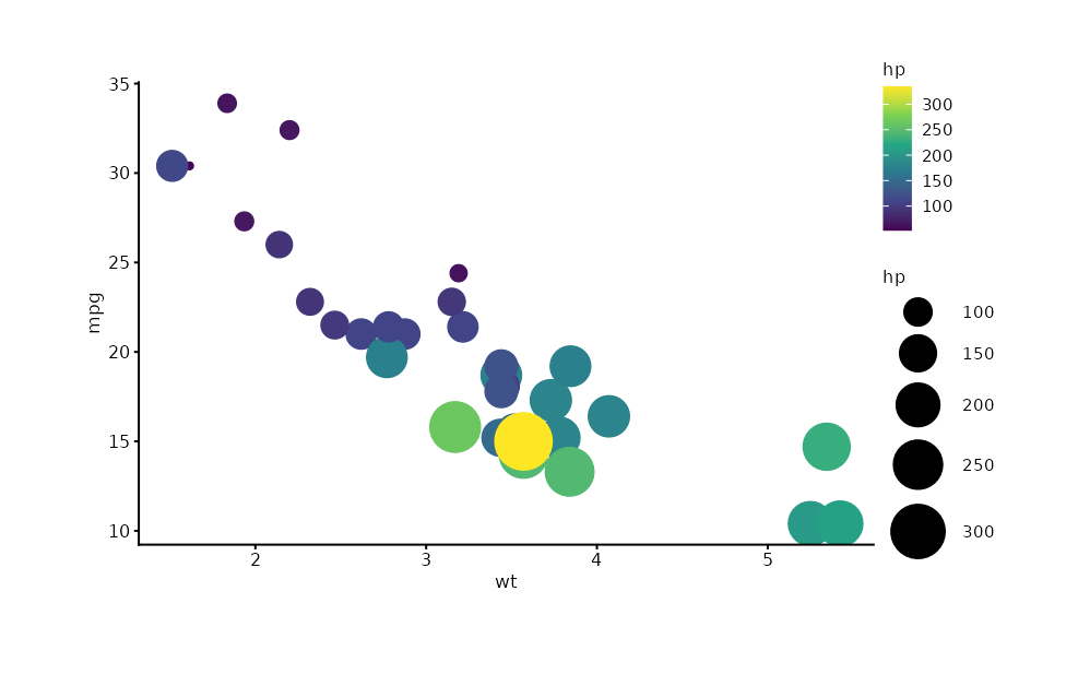
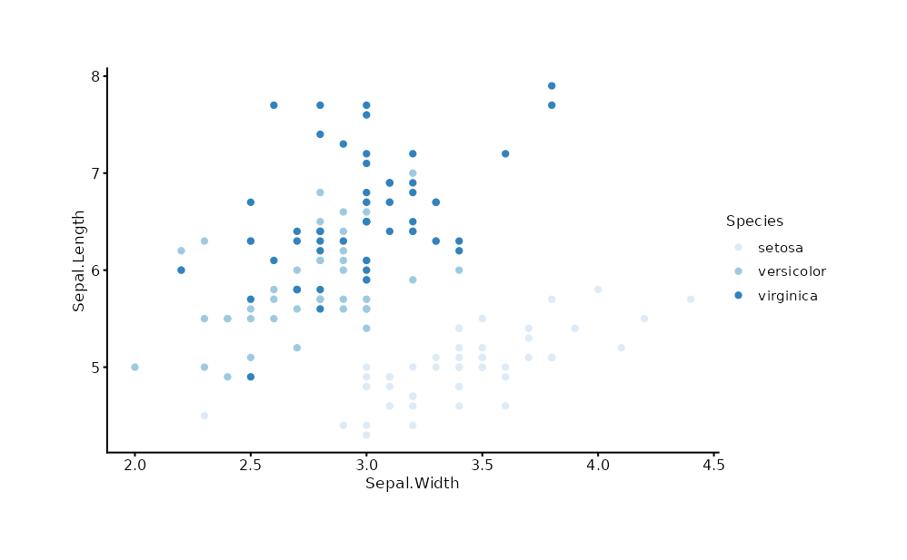
iris |>
  plotit(encode(x = Sepal.Width, y = Sepal.Length, colour = Species)) |>
  mark_point() |>
  scale_color(range = "brewer")
#> Scale for colour is already present.
#> Adding another scale for colour, which will replace the existing scale.