Statistical ribbon layer — mark

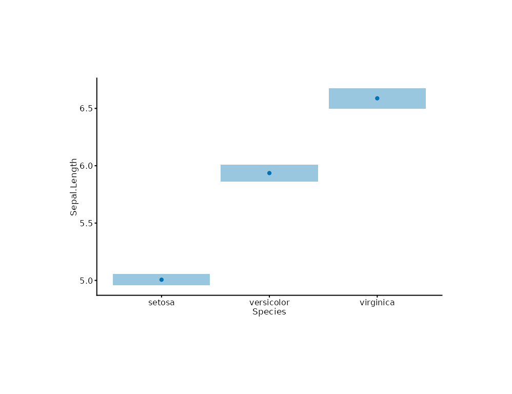
Draws an interval band. This is a syntax-sugar composite mark over geom_ribbon:

Usage

mark_ribbon(
  plot,
  mapping = NULL,
  data = NULL,
  position = NULL,
  ...,
  stat = "identity",
  level = 0.95,
  ci_method = c("normal", "boot"),
  seed = NULL,
  alpha = NULL,
  width = 0.9,
  rasterize = FALSE,
  rasterize_dpi = 300,
  rasterize_dev = "cairo"
)

Arguments

plot: A plotit object
mapping: Optional aesthetics: x plus ymin/ymax for stat = "identity", or x (group) + y (value) for a statistical entity.
data: Optional data for this layer
position: Position adjustment.
...: Other arguments passed to geom_ribbon
stat: Statistical entity: "identity" (pre-computed band) or "mean_sem" / "mean_sd" / "mean_range" / "mean_ci95" (per-group aggregation of y; shares the engine with mark_errorbar()).
level: Confidence level for stat = "mean_ci95", in (0, 1).
ci_method: "normal" (t-based approximation) or "boot" (percentile bootstrap; requires seed).
seed: RNG seed for ci_method = "boot".
alpha: Band fill opacity; NULL (default) uses the statistical token alpha_ci (0.4), matching tidyplots ribbons behind points and lines.
width: On a discrete x axis, the band occupies this share of each category slot (default 0.9); a statistical entity becomes one slot-width rectangle band per group, filled by the grouping channel.
rasterize: If TRUE, rasterize via ggrastr::rasterise().
rasterize_dpi: DPI for rasterization (default 300).
rasterize_dev: Graphics device for rasterization (default "cairo").

Value

Modified plotit object

Details

Equivalent expansion:


  stat = "identity"  is  mark_area()'s interval routing (ymin/ymax from
                     the data, no aggregation)
  stat = "mean_sem"  is  stat_summary(fun.data = mean_sem, geom = "ribbon")
                     (tidyplots add_sem_ribbon is the same shape)

References

Vega-Lite: Errorband (extent: stderr <-> sem, stdev <-> sd, ci <-> ci95)

tidyplots: add_sem_ribbon() / add_ci95() (same aggregation shapes)

Examples

fit <- stats::loess(mpg ~ wt, data = mtcars)
band <- data.frame(
  wt = mtcars$wt,
  fit = stats::predict(fit),
  se = stats::predict(fit, se = TRUE)$se.fit
)
band$lo <- band$fit - 1.96 * band$se
band$hi <- band$fit + 1.96 * band$se
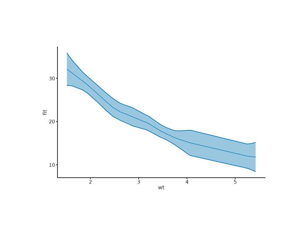
plotit(band, encode(x = wt, ymin = lo, ymax = hi)) |>
  mark_ribbon() |>
  mark_line(mapping = encode(x = wt, y = fit))


# statistical entity: mean +- sem per group from raw y
plotit(iris, encode(x = Species, y = Sepal.Length)) |>
  mark_ribbon(stat = "mean_sem") |>
  mark_point(stat = "summary", fun = "mean")