Chord layout

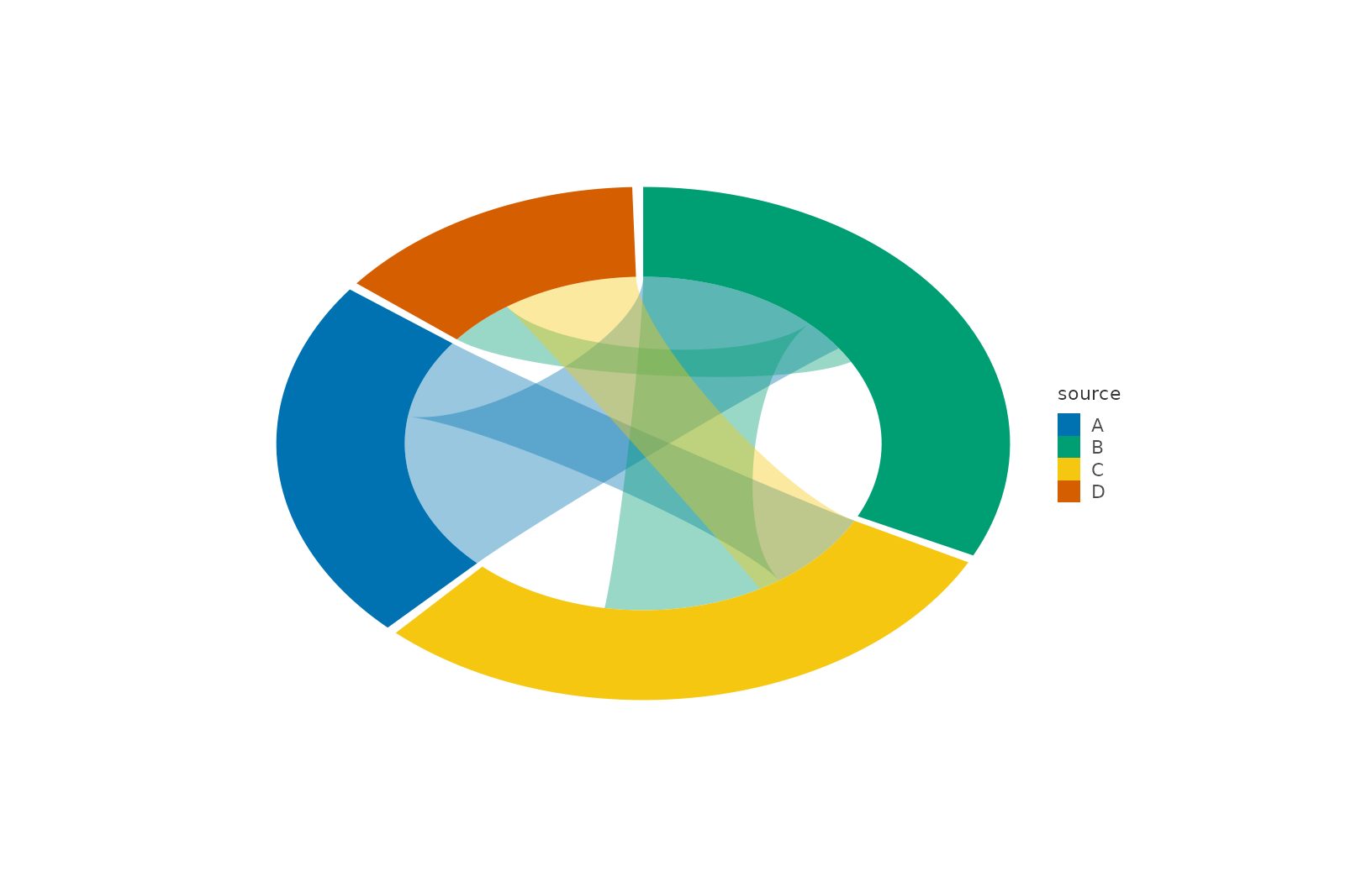
Circular chord layout: nodes become annular sectors on a ring whose angular spans are proportional to total incident flow; edges become closed bezier bands crossing the interior. Emits four tables:

Usage

layout_chord(
  plot,
  inner_radius = 0.65,
  pad_angle = 0.03,
  n_points = 60,
  curvature = 0.35,
  order_by = c("total", "appearance")
)

Arguments

plot

A plotit object holding graph data, or a bare plotit_graph.

inner_radius

Inner radius of the ring, (0, 1).

pad_angle

Gap between sectors in radians.

n_points

Samples per boundary chain of each polygon.

curvature

Inward bowing of bands, [0, 0.95].

order_by

"total" sorts sectors by descending flow; "appearance" keeps first-appearance order.

Value

A modified plotit object (pipeline form), or a new plotit_graph with arcs/ribbons tables when called on raw graph data.

Details

• nodes – original attributes plus flow_total, arc angles (arc_lo/arc_hi) and xc/yc label anchors outside the ring;

• edges – untouched topology rows;

• arcs – long-form sector polygons (.arc_id, x, y, node attrs) rendered with mark_polygon(data = ~arcs, group = .arc_id);

• ribbons – long-form band polygons (.ribbon_id, x, y, edge attrs) rendered with mark_polygon(data = ~ribbons, group = .ribbon_id).

Duplicate (source, target) pairs are summed into a single band. Sectors are ordered by descending total flow by default; use order_by = "appearance" to keep input order. Fully deterministic.

Examples

e <- data.frame(
  source = c("A", "A", "B", "B", "C"),
  target = c("B", "C", "C", "D", "D"),
  value  = c(10, 5, 8, 3, 6)
)
g <- as_graph(e) |> layout_chord()
g$nodes[, c("id", "flow_total")]
#>   id flow_total
#> 1  A         15
#> 2  B         21
#> 3  C         19
#> 4  D          9

as_graph(e) |>
  plotit() |>
  layout_chord() |>
  mark_polygon(
    data = ~ribbons,
    encode(fill = source, group = .ribbon_id),
    alpha = 0.4
  ) |>
  mark_polygon(
    data = ~arcs,
    encode(fill = id, group = .arc_id)
  )