Empirical CDF layer — mark

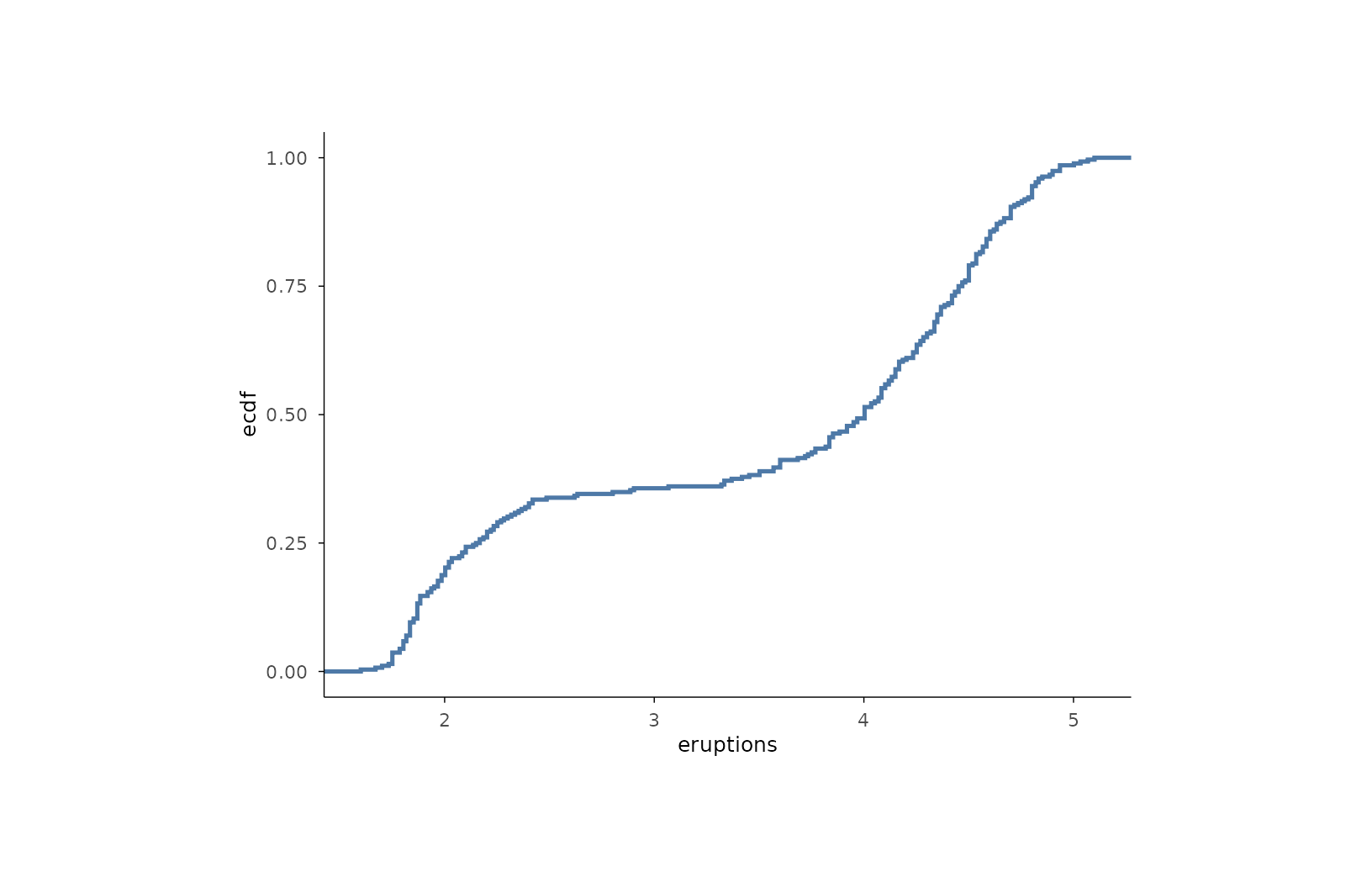
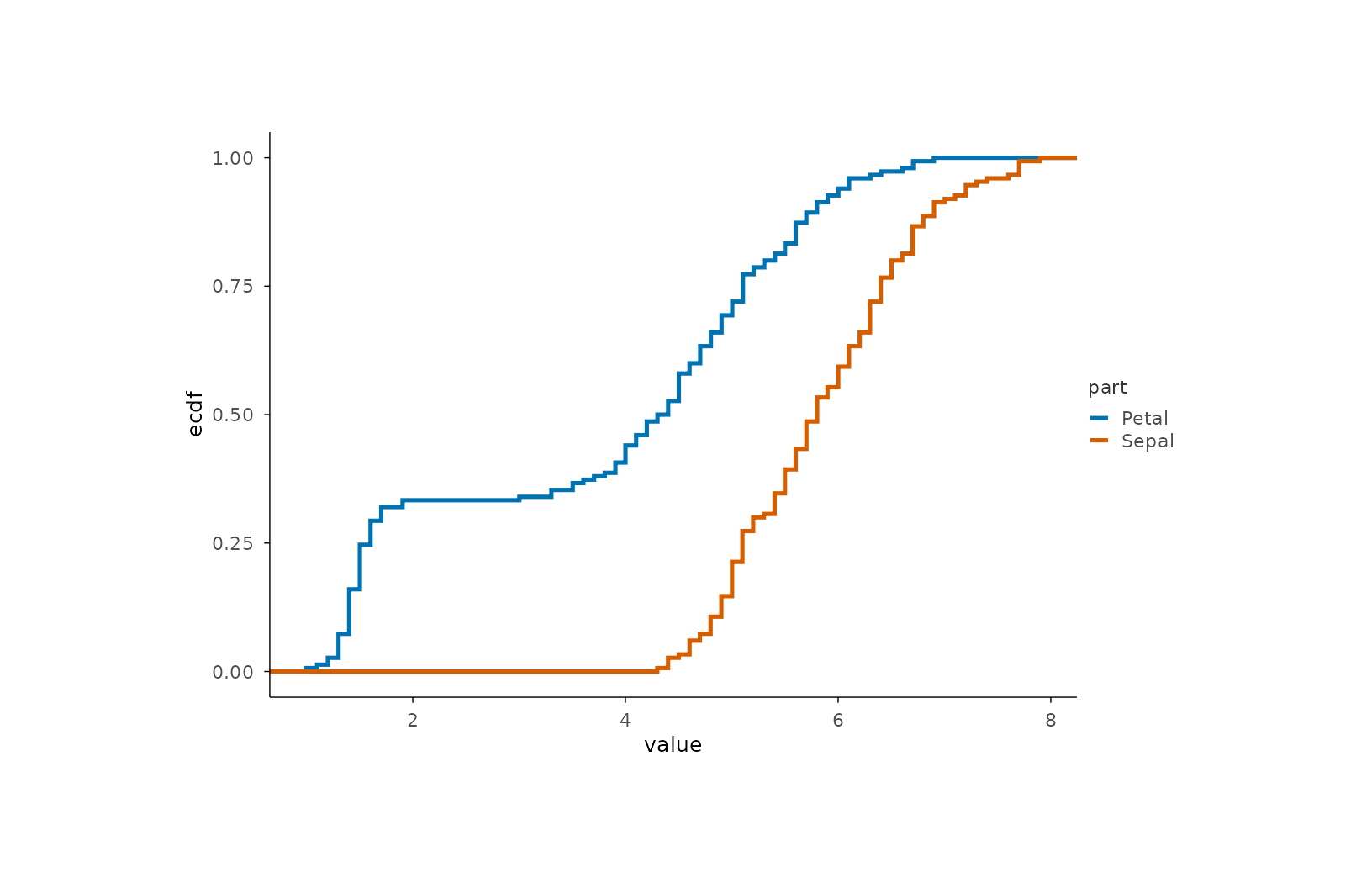
Plots the empirical cumulative distribution function as a stair step. A distribution view with no binning parameter to choose: every point is exactly represented, and group comparisons (quantiles, shifts, tails) are easy to read.

Usage

mark_ecdf(
  plot,
  mapping = NULL,
  data = NULL,
  position = NULL,
  ...,
  n = 1000,
  rasterize = FALSE,
  rasterize_dpi = 300,
  rasterize_dev = "cairo"
)

Arguments

plot: A plotit object
mapping: Optional new aesthetics (x is the sample)
data: Optional data for this layer
position: Position adjustment.
...: Other arguments passed to the underlying step layer
n: Oversampling factor for the step function (default 1000; use Inf for the exact step function).
rasterize: If TRUE, rasterize via ggrastr::rasterise().
rasterize_dpi: DPI for rasterization (default 300).
rasterize_dev: Graphics device for rasterization (default "cairo").

Value

Modified plotit object

References

Observable Plot: Plot.ecdf

Vega-Lite: line/step with cumulative window transform

Examples

plotit(faithful, encode(x = eruptions)) |> mark_ecdf()


# ECDF comparison
df <- data.frame(
  value = c(iris$Sepal.Length, iris$Petal.Length),
  part = rep(c("Sepal", "Petal"), each = 150)
)
plotit(df, encode(x = value, colour = part)) |>
  mark_ecdf()