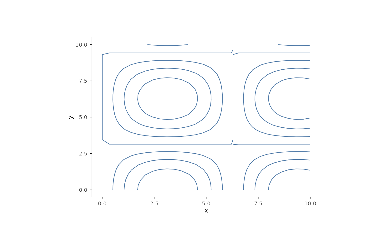
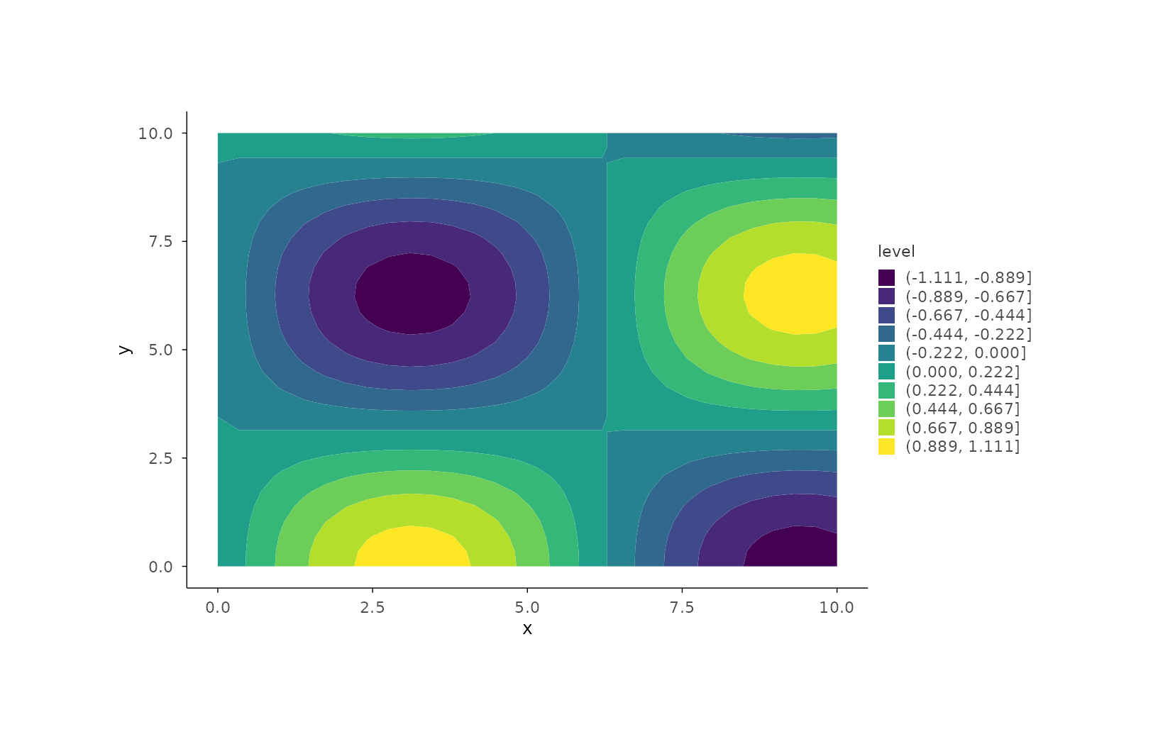
Contour layer for 2D scalar fields — mark

Draws contour lines of a 2D scalar field: the data must carry a z aesthetic (value at each x/y grid point). Use filled = TRUE for banded fills. Where mark_density_2d() estimates density from points, mark_contour() renders an observed field (elevation, temperature, a fitted surface).

Usage

mark_contour(
  plot,
  mapping = NULL,
  data = NULL,
  position = NULL,
  ...,
  filled = FALSE,
  bins = NULL,
  breaks = NULL,
  rasterize = FALSE,
  rasterize_dpi = 300,
  rasterize_dev = "cairo"
)

Arguments

plot: A plotit object
mapping: Optional new aesthetics (must include x, y, z)
data: Optional data for this layer
position: Position adjustment.
...: Other arguments passed to the underlying geom
filled: If TRUE, draw filled contour bands via geom_contour_filled; otherwise contour lines via geom_contour.
bins: Number of contour bins.
breaks: Numeric vector of exact contour levels; overrides bins.
rasterize: If TRUE, rasterize via ggrastr::rasterise().
rasterize_dpi: DPI for rasterization (default 300).
rasterize_dev: Graphics device for rasterization (default "cairo").

Value

Modified plotit object

Details

Filled bands map fill to a computed level factor owned by this closed statistical mark; the band scale defaults to discrete viridis and can be replaced by chaining scale_fill() afterwards.

References

AntV G2: Contour

Observable Plot: Plot.contour

Examples

df <- expand.grid(x = seq(0, 10, length.out = 30), y = seq(0, 10, length.out = 30))
df$z <- with(df, sin(x / 2) * cos(y / 2))
plotit(df, encode(x = x, y = y, z = z)) |>
  mark_contour(breaks = seq(-1, 1, by = 0.25))


plotit(df, encode(x = x, y = y, z = z)) |>
  mark_contour(filled = TRUE, bins = 10)